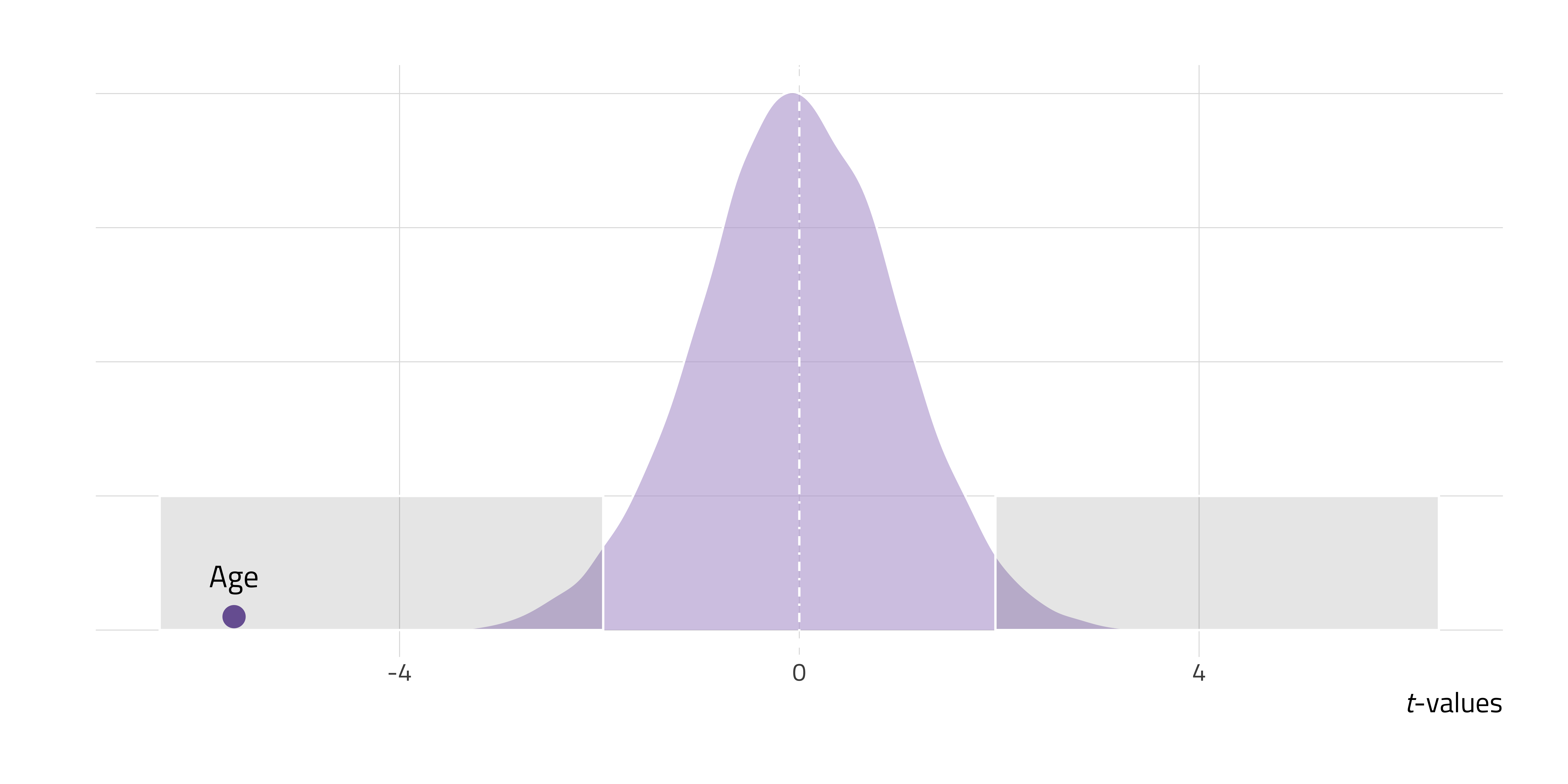
Week 5
Data Analysis

Soci—316

Sakeef M. Karim
Amherst College

SOCIAL RESEARCH

Classical Statistics—
September 29^th

Updates

Memo on Research Interests

Brief comments vis-à-vis your research memos are
available through Moodle.

Updates

Qualtrics Survey Assignment

Qualtrics Survey Assessment Deadline

Your Qualtrics survey assignments are due by
8:00 PM on Friday, Octobr 9^th.

Qualtrics Survey Assessment

High-Level Overview Regressions as Prediction Machines

A Basic Assertion

We should treat regressions as
counterfactual prediction machines.

Link to Article

A Basic Assertion

For Future Reference

• marginaleffects
• clarify

Full Page

Full Page

A Basic Assertion

Today, we’ll explore this idea—and work to demystify regressions—using a
basic example.

Our Case

Image source

en.wikipedia.org/wiki/—

Loading the article

Our Task

To predict the probability of surviving the sinking of the Titanic as a function of predictors like age, sex and
passenger class.

P(\text{Survival} = 1 \mid X) = \beta_0 + X\beta + \varepsilon

Our Strategy

We’re going to estimate a
linear probability model.

Our Strategy

Caveat Emptor

Using a linear probability model (LPM) to predict a binary outcome can produce predicted probabilities—P(Y=1\mid X)—that fall outside the [0, 1] interval.

We’re going to fit one anyway
(cf. Hippel 2015).

A Simple Bivariate Model

Our Truncated Sample

library(tidyverse)

titanic <- carData::TitanicSurvival |> 
           rownames_to_column(var = "name") |> 
           as_tibble() |> 
           mutate(survived = as.numeric(survived) - 1) 

set.seed(905)

titanic_subset <- titanic |> 
                  slice_sample(n = 3, by = passengerClass) |> 
                  select(name, survived, age)

titanic_subset

# A tibble: 9 × 3
  name                            survived   age
  <chr>                              <dbl> <dbl>
1 Aubart, Mme. Leontine Pauline          1    24
2 Stone, Mrs. George Nelson (Mart        1    62
3 Cardeza, Mr. Thomas Drake Marti        1    36
4 Buss, Miss. Kate                       1    36
5 Smith, Miss. Marion Elsie              1    40
6 Hocking, Mr. Richard George            0    23
7 Cohen, Mr. Gurshon Gus                 1    18
8 Cribb, Mr. John Hatfield               0    44
9 Skoog, Miss. Mabel                     0     9

Our First Model

P(\text{Survival} = 1 \mid X) = \beta_0 + \beta_1\text{age} + \varepsilon

We’re modelling the probability of survival as a function of age.

Our First Model

To fit this model, we need to calculate the slope and intercept parameters—that is, \beta_0 and \beta_1\text{age}, respectively.

Slopes can be derived using the following formula:

b = \frac{\sum{(X - \bar{X})(Y - \bar{Y})}}{\sum{(X - \bar{X})^2}}

Intercepts can be calculated as follows:

\alpha = \bar{Y} - b\bar{X}

Our First Model

Plugging in Our Values

• Step 1: Slope
• Step 2: Intercept

Y	X	X - \bar{X}	Y - \bar{Y}	(X - \bar{X})(Y - \bar{Y})	(X - \bar{X})^2
1	24	−8.44	0.33	−2.81	71.31
1	62	29.56	0.33	9.85	873.53
1	36	3.56	0.33	1.19	12.64
1	36	3.56	0.33	1.19	12.64
1	40	7.56	0.33	2.52	57.09
0	23	−9.44	−0.67	6.30	89.20
1	18	−14.44	0.33	−4.81	208.64
0	44	11.56	−0.67	−7.70	133.53
0	9	−23.44	−0.67	15.63	549.64
		\sum (X - \bar{X}) = 0	\sum (Y - \bar{Y}) = 0	\sum (X - \bar{X})(Y - \bar{Y}) = 21.33	\sum (X - \bar{X})^2 = 2008.22

\beta_1 = \frac{\sum (X - \bar{X})(Y - \bar{Y})}{\sum (X - \bar{X})^2}

{} = \frac{21.33}{2008.22} \approx 0.0106

\beta_0 = 0.667 - (0.0106 \times 32.44) \approx 0.3220

Our first LPM can therefore be summarized as follows:

\hat{P}(\text{Survived} = 1) = 0.3220 + 0.0106 \cdot \text{age} + \varepsilon

Our First Model

Plugging in Our Values

We can use programs like to streamline hand calculations.

library(tidyverse)

titanic_subset |> mutate(# Averages
                         mean_y = mean(survived),
                         mean_x = mean(age),
                         # To establish covariation between x and y
                         # Deviations from average, x
                         x_minus_mean_x = age - mean(age),
                         # Corresponding y value--deviations from average
                         y_minus_mean_y = survived - mean(mean_y),
                         # Tapping co-movement
                         slope_numerator = x_minus_mean_x * y_minus_mean_y,
                         # Squared residuals, positive values are yielded
                         slope_denominator = x_minus_mean_x^2) |> 
                         # Putting it all together
                  mutate(# Summing up the values for the numerator ...
                         slope_numerator = sum(slope_numerator),
                         # And the denominator ...
                         slope_denominator = sum(slope_denominator),
                         # Yielding the slope estimate
                         slope = slope_numerator/slope_denominator,
                         # Which allows us to "solve" for the intercept:
                         intercept = mean_y - slope * mean_x) |> 
                  select(intercept, slope) |> 
                  distinct()

# A tibble: 1 × 2
  intercept  slope
      <dbl>  <dbl>
1     0.322 0.0106

And thankfully, get around doing hand calculations in the first place.

lm(survived ~ age, data = titanic_subset)

Call:
lm(formula = survived ~ age, data = titanic_subset)

Coefficients:
(Intercept)          age  
    0.32201      0.01062  

Let’s Use Our Model

A Case Study

Kate Buss was 36 years old when the Titanic sank.

# A tibble: 1 × 3
  name             survived   age
  <chr>               <dbl> <dbl>
1 Buss, Miss. Kate        1    36

We can compute her probability of survival Using our clearly misspecified model. as follows:

0.32201 + (0.01062 * 36) 

[1] 0.70433

Or we can use functions to generate these predictions for us.

survival_truncated <- lm(survived ~ age, data = titanic_subset) 

titanic_subset |> 
# No measures of uncertainty here
mutate(estimate = predict(survival_truncated)) |> 
slice(4)

# A tibble: 1 × 4
  name             survived   age estimate
  <chr>               <dbl> <dbl>    <dbl>
1 Buss, Miss. Kate        1    36    0.704

Let’s Use Our Model

Counterfactual Predictions—With Our Truncated Sample

library(marginaleffects)

avg_predictions(survival_truncated, variables = "age") |> 
as_tibble() |> 
ggplot(mapping = aes(x = age, y = estimate)) +
geom_line(colour = "#b7a5d3", linewidth = 1.5) +
geom_ribbon(mapping = aes(ymin = conf.low,
                          ymax = conf.high),
            fill = "#b7a5d3",
            alpha = 0.35) +
theme_bw()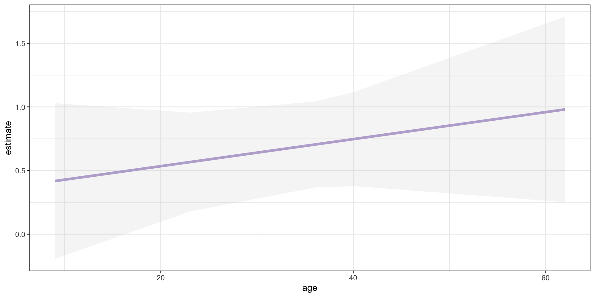

Let’s Use Our Model

Counterfactual Predictions—With the Full Sample

survival_full <- lm(survived ~ age, data = titanic) 

avg_predictions(survival_full, variables = "age") |> 
as_tibble() |> 
ggplot(mapping = aes(x = age, y = estimate)) +
geom_line(colour = "#b7a5d3", linewidth = 1.5) +
geom_ribbon(mapping = aes(ymin = conf.low,
                          ymax = conf.high),
            fill = "#b7a5d3",
            alpha = 0.35) +
theme_bw()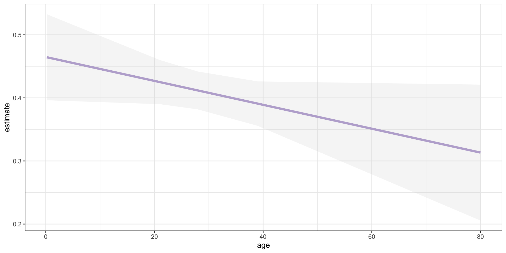

Let’s Use Our Model

Uh-oh.
Our initial model painted a misleading portrait.

Adding More Predictors

Updating the Full Model

update(survival_full, . ~ . + sex + passengerClass) |> 
summary()

Call:
lm(formula = survived ~ age + sex + passengerClass, data = titanic)

Residuals:
     Min       1Q   Median       3Q      Max 
-1.09442 -0.24408 -0.08375  0.23289  0.99397 

Coefficients:
                    Estimate Std. Error t value Pr(>|t|)    
(Intercept)        1.1049549  0.0438210  25.215  < 2e-16 ***
age               -0.0052695  0.0009316  -5.656 2.00e-08 ***
sexmale           -0.4914131  0.0255520 -19.232  < 2e-16 ***
passengerClass2nd -0.2113738  0.0348568  -6.064 1.85e-09 ***
passengerClass3rd -0.3703874  0.0325039 -11.395  < 2e-16 ***
---
Signif. codes:  0 '***' 0.001 '**' 0.01 '*' 0.05 '.' 0.1 ' ' 1

Residual standard error: 0.3913 on 1041 degrees of freedom
  (263 observations deleted due to missingness)
Multiple R-squared:  0.3691,    Adjusted R-squared:  0.3667 
F-statistic: 152.3 on 4 and 1041 DF,  p-value: < 2.2e-16

Updating the Full Model

\begin{align*} \hat{P}(\text{Survived} = 1) = 1.105 - 0.00527 \cdot \text{age} - 0.4914 \cdot \text{sex}_\text{male} \\ - 0.2114 \cdot \text{class}_\text{2nd} - 0.3704 \cdot \text{class}_\text{3rd} + \varepsilon \end{align*}

Call:
lm(formula = survived ~ age + sex + passengerClass, data = titanic)

Coefficients:
      (Intercept)                age            sexmale  passengerClass2nd  
         1.104955          -0.005269          -0.491413          -0.211374  
passengerClass3rd  
        -0.370387  

We’re now modelling the probability of survival as a function of
age, sex and passenger class.

A Group Exercise

Making Predictions

Here are three passengers selected at random:

# A tibble: 3 × 5
  name                            survived sex     age passengerClass
  <chr>                              <dbl> <fct> <dbl> <fct>         
1 Veal, Mr. James                        0 male     40 2nd           
2 Petersen, Mr. Marius                   0 male     24 3rd           
3 Johnson, Master. Harold Theodor        1 male      4 3rd           

In small groups, calculate the probability of survival for each passenger.

Call:
lm(formula = survived ~ age + sex + passengerClass, data = titanic)

Coefficients:
      (Intercept)                age            sexmale  passengerClass2nd  
         1.104955          -0.005269          -0.491413          -0.211374  
passengerClass3rd  
        -0.370387  

The Solution

# A tibble: 3 × 2
  name                            estimate
  <chr>                              <dbl>
1 Veal, Mr. James                    0.191
2 Petersen, Mr. Marius               0.117
3 Johnson, Master. Harold Theodor    0.222

The Hand Calculation

x <- c(24, 4)

c(1.104955 - 0.491413 - 0.211374 - (40 * 0.005269),
  map_dbl(x, ~  1.104955 - 0.491413 - 0.370387 - (. * 0.005269)))

[1] 0.191408 0.116699 0.222079

A Note About Uncertainty

Meaning in the Stars

modelsummary::modelsummary(survival_full,
                           stars = TRUE,
                           gof_map = NA,  
                           statistic = NULL)

	(1)
+ p < 0.1, * p < 0.05, ** p < 0.01, *** p < 0.001
(Intercept)	1.105***
age	-0.005***
sexmale	-0.491***
passengerClass2nd	-0.211***
passengerClass3rd	-0.370***

Standard Errors

SE(\hat{\beta}) = \sqrt{\frac{\hat{\sigma}^2}{\sum_{i = 1}^n (x_i- \bar{x})^2}}

Parameter estimates based on our full model.

# A tibble: 1 × 5
  term  estimate std.error statistic      p.value
  <chr>    <dbl>     <dbl>     <dbl>        <dbl>
1 age   -0.00527  0.000932     -5.66 0.0000000155

Hypothesis Testing

In Standard OLS Settings

t = \frac{\hat{\beta} - \color{#856cb0}{\beta_{H_\theta}}}{SE(\hat{\beta})}

Hypothesis Testing

In Standard OLS Settings

t = \frac{\hat{\beta} - \color{#856cb0}{\beta_{H_0}}}{SE(\hat{\beta})}

survival_full |> 
broom::tidy() |> 
filter(term == "age") |> 
mutate(manual_statistic = (estimate - 0)/std.error,
       .after = statistic)

# A tibble: 1 × 6
  term  estimate std.error statistic manual_statistic      p.value
  <chr>    <dbl>     <dbl>     <dbl>            <dbl>        <dbl>
1 age   -0.00527  0.000932     -5.66            -5.66 0.0000000200

Hypothesis Testing

In Standard OLS Settings

Statistical Significance

According to Your Textbook

A result is statistically significant at the 5% level when the corresponding parameter is distinguishable from zero using 5% as the rejection threshold. Conversely, a result is not statistically significant at the 5% level when the corresponding parameter is not distinguishable from zero using 5% as the rejection threshold.

(Llaudet and Imai 2023:215, EMPHASIS ADDED)

Another Group Exercise

Predictions and ATEs

As Llaudet and Imai (2023) note, we can use simple linear models to approximate the difference-in-means estimator and derive our key estimand, the \widehat{\textit{ATE}}.

In small groups, discuss how conceptualizing regressions as counterfactual prediction machines can help us understand what the \widehat{\textit{ATE}} represents.

Qualtrics Surveys

Refine Your Survey Instrument

For the rest of today’s session, please work on your
Qualtrics survey assignment.

Machine Learning—
October 1^st

A New Deadline?

Qualtrics Survey Assignment

Assignment instructions are online.

Full Page

Machine Learning:
What Is It?

Some Definitional Work

Defining Machine Learning In your own words, define machine learning.

5:00

0 words

Some Concrete Definitions

Grimmer and colleagues (2021:396)

A class of flexible algorithmic and statistical techniques for prediction and dimension reduction.

Molina and Garip (2019:28)

A way to learn from data and estimate complex functions that discover representations of some input (X), or link the input to an output (Y) in order to make predictions on new data.

Supervised Machine Learning (SML)

High-Level Overview

Once deployed, SML algorithms learn the complex patterns linking X—a set of features Independent variables or predictors. —to a target variable Outcome or dependent variable. , Y.

The goal of SML is to optimize predictions—i.e., to find functions or algorithms that offer substantial predictive power when confronted with
new or unseen data.

Examples

SML algorithms include, but are not limited to, logistic regressions, random forests, ridge regressions, support vector machines and neural networks.

Supervised Machine Learning (SML)

High-Level Overview

A quick note on terminology:

• Regression
• Classification

If a target variable is quantitative, we are dealing with a regression problem.

If a target variable is qualitative, we are dealing with a classification problem.

Supervised Machine Learning (SML)

An Illustration

# A tibble: 80,000 × 6
   fruit      shape       weight_g colour texture origin    
   <chr>      <chr>          <int> <chr>  <chr>   <chr>     
 1 apple      spherical        150 red    crispy  china     
 2 banana     curved           120 yellow creamy  ecuador   
 3 orange     spherical        148 orange juicy   egypt     
 4 watermelon spherical       4500 green  juicy   spain     
 5 strawberry conical           13 red    juicy   mexico    
 6 grape      spherical          5 green  juicy   chile     
 7 mango      ellipsoidal      240 yellow juicy   india     
 8 pineapple  conical         2100 yellow juicy   costa rica
 9 apple      spherical        140 green  crispy  usa       
10 banana     curved           110 yellow creamy  ecuador   
# ℹ 79,990 more rows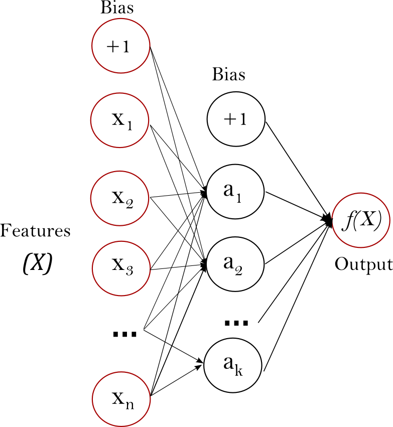

scikit-learn

# A tibble: 1 × 6
  fruit shape   weight_g colour texture origin
  <chr> <chr>      <int> <chr>  <chr>   <chr> 
1 <NA>  conical        6 red    juicy   china 

strawberry71%

grape21%

orange5%

apple3%

banana0%

watermelon0%

mango0%

pineapple0%

strawberry71% probability

Flaticon

Unsupervised Machine Learning (UML)

High-Level Overview

UML algorithms search for a representation of the inputs/features that is more useful than X itself (Molina and Garip 2019).

With UML, analysts mine for hidden structure or latent patterns in high-dimensional space.

What does this mean, exactly?

Unsupervised Machine Learning (UML)

High-Level Overview

With UML, there is no observed outcome variable Y—or target—to supervise the estimation process. Instead, we only have inputs.

The primary goal in UML is to develop a lower-dimensional representation of complex data by inductively learning from the
interrelationships among inputs.

Common Strategies

Reducing a vector of features to a small set of scales (e.g., via principal component analysis) or dividing a sample into a small number of hidden groups (e.g., via k-means clustering).

Unsupervised Machine Learning (UML)

An Illustration

V-Party Variable Underlying question

Anti-Elitismv2paanteli

How important is anti-elite rhetoric for this party?

People-Centrismv2papeople

Do leaders of this party glorify the ordinary people and identify themselves as part of them?

Cultural Chauvinismv2paculsup

To what extent does the party leadership promote the cultural superiority of a specific social group or the nation as a whole?

Minority Rightsv2paminor

According to the leadership of this party, how often should the will of the majority be implemented even if doing so would violate the rights of minorities?

Political Pluralismv2paplur

Prior to this election, to what extent was the leadership of this political party clearly committed to free and fair elections with multiple parties, freedom of speech, media, assembly and association?

Demonization of Opponentsv2paopresp

Prior to this election, have leaders of this party used severe personal attacks or tactics of demonization against their opponents?

Rejection of Political Violencev2paviol

To what extent does the leadership of this party explicitly discourage the use of violence against domestic political opponents?

Unsupervised Machine Learning (UML)

An Illustration

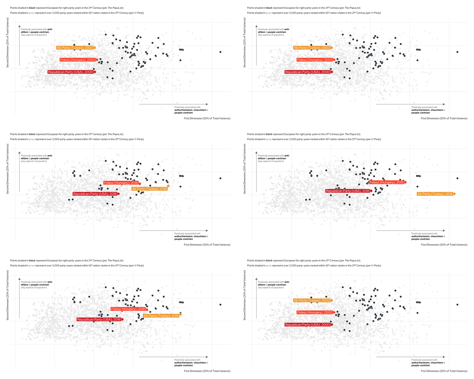
Karim and Lukk’s The Radicalization of Mainstream Parties in the 21^st Century

The Two “Cultures”

As Grimmer and colleagues note (2021:397, EMPHASIS ADDED) note, “machine learning is as much a culture defined by a distinct set of values and tools as it is a set of algorithms.”

The Two “Cultures”

This point has, of course, been made elsewhere.

Full Article

Note

The terms generative and predictive (as opposed to data and algorithmic) come from David Donoho’s (2017) 50 Years of Data Science.

Machine Learning vs Classical Statistics

The Two Cultures

\hat{\beta} Generative Classical statistics

Inferring relationships between X and Y

• Interpretability
• Emphasis on uncertainty
• Explanatory power

• Bounded by statistical assumptions
• Inattention to variance across samples

\hat{y} Predictive Machine learning

Generating accurate predictions of Y

• Predictive power
• Can simplify high-dimensional data
• Relatively unbeholden to statistical assumptions

• Inattention to explanatory processes
• Opaque links between X and Y

Note

To be sure, the putative strengths and weaknesses of these modelling “cultures” have been hotly debated.

The Affordances of Machine Learning

Advances in machine learning can provide empirical leverage to social scientists and sharpen social theory in one fell swoop.

Lundberg, Brand and Jeon (2022), for instance, argue that embracing machine learning can help social scientists in at least four ways.

Four Key Benefits

• By amplifying human coding
• By summarizing complex data structures
• By relaxing statistical assumptions
• By targeting researcher attention

Just Inductive?

ML is often associated with induction. van Loon (2022) argues that SML algorithms can help us deductively resolve predictability hypotheses, too.

Key Terms and Concepts in the SML Setting

Bias-Variance Tradeoff

Wikimedia Commons

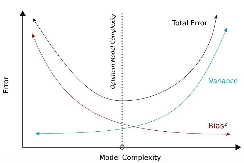
Emerges when we build SML algorithms that fail to sufficiently map the patterns—or pick up the empirical signal—linking X and Y. Think: underfitting.

Arises when our algorithms not only pick up the signal linking X and Y, but some of the noise in our data as well. Think: overfitting.

To strike the optimal balance between bias and variance.

Training, Validation and Testing

In an SML setting, we want to reduce our algorithm’s generalization or test error—i.e., “the prediction error of a model on new data” (Molina and Garip 2019).

Training, Validation and Testing

To arrive at an estimate of our model’s performance, we can (randomly) partition our global sample of observations into disjoint sets or subsamples.

• We can use a training set to fit our algorithm—to find weights (or coefficients), recursively split the feature space to grow decision trees and so on.
• Training data should constitute the largest of our three disjoint sets.

• We can use a validation set to find the right estimator out of a series of candidate algorithms—or select the best-fitting parameterization of a single algorithm.
• Using both training and validation sets can be costly: data sparsity can amplify variance.
• Thus, when limited to smaller samples, analysts often combine training and validation—say, by recycling training data for model tuning and selection.

• We can use a testing set to generate a measure of our model’s predictive accuracy (e.g., the F1 score for classification problems)—or to derive our generalization error.
• This subsample is used only once (to report the performance metric); put another way, it cannot be used to train, tune or select our algorithm.

k-Fold Cross-Validation

Stylized example of five-fold cross-validation

Test Train Train Train Train Train Test Train Train Train Train Train Test Train Train Train Train Train Test Train Train Train Train Train Test

Evaluation₁ Evaluation₂ Evaluation₃ Evaluation₄ Evaluation₅

Performance 15 5∑i=1 Evaluation_i

Detailed Overview

• Unlike standard train/test splits, v or k-fold cross-validation lets us learn from all our data.

• k-fold cross-validation proceeds as follows:

  • We randomly divide our overall sample into k subsets or folds.
  • We train our algorithm on k - 1 folds, holding just one group out for model assessment.
  • We repeat this process k times—every fold is held out once and used to fit the model k - 1 times.
  • We then pool or average the evaluation metrics (e.g., predictive accuracy) for all the held-out runs.

• Stratified k-fold cross-validation ensures that the distribution of class labels—or for numeric targets, the mean—is relatively constant across folds.

Three Quick Examples

Gender Typicality

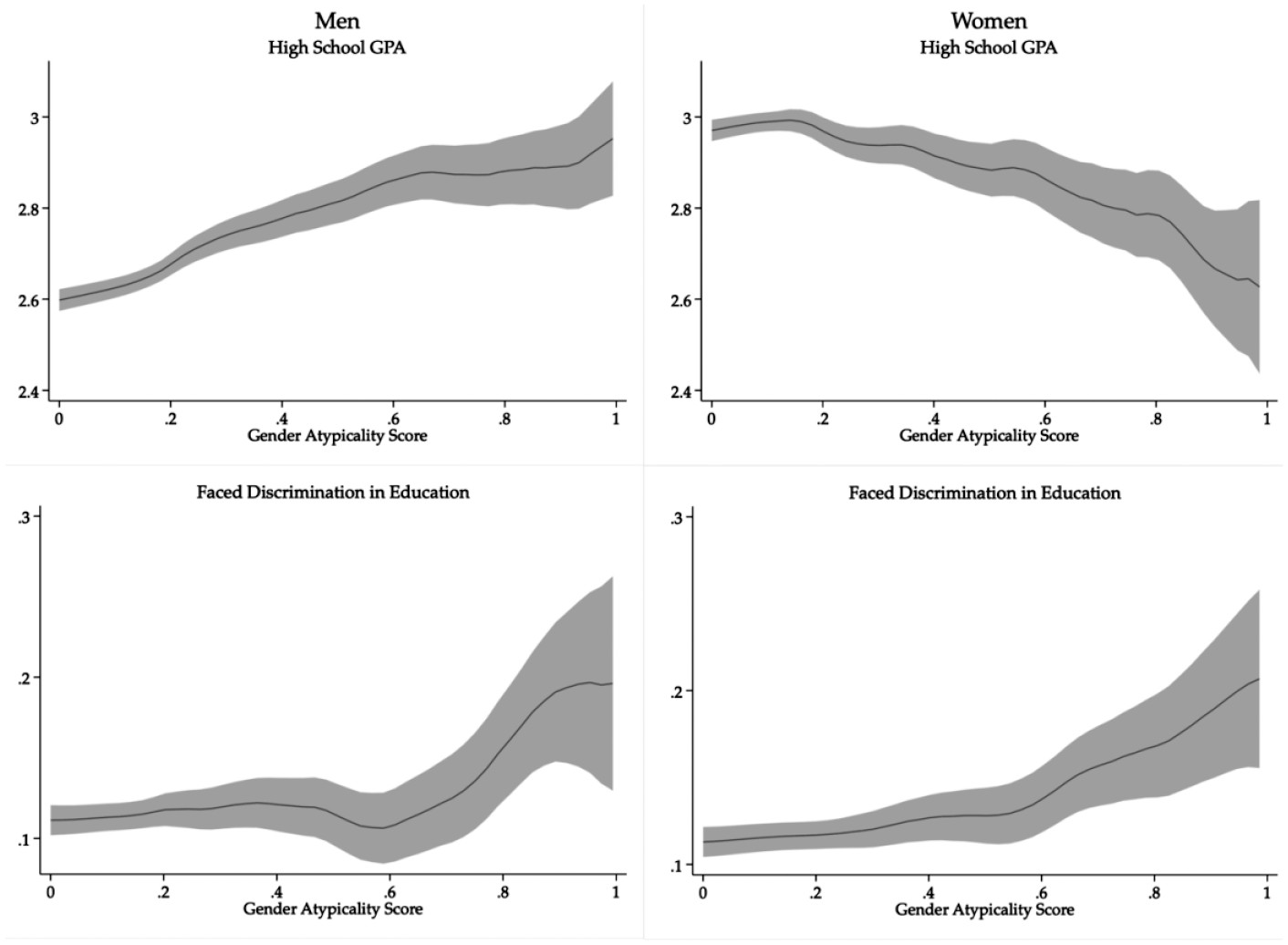
Figure 8 from Mittleman (2022).

Gendered Stereotypes in Print Media

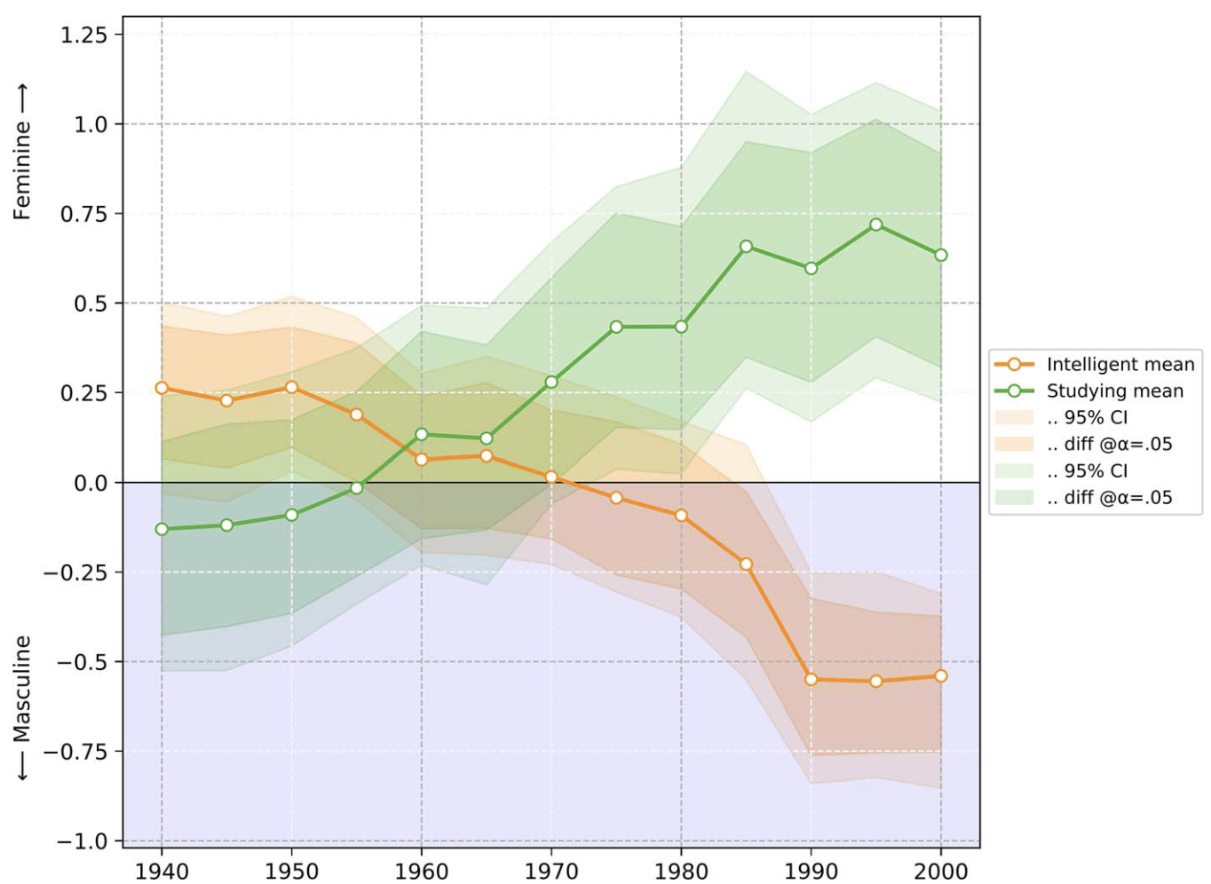
Figure 8  from Boutyline and colleagues (2023)

Acculturative Change

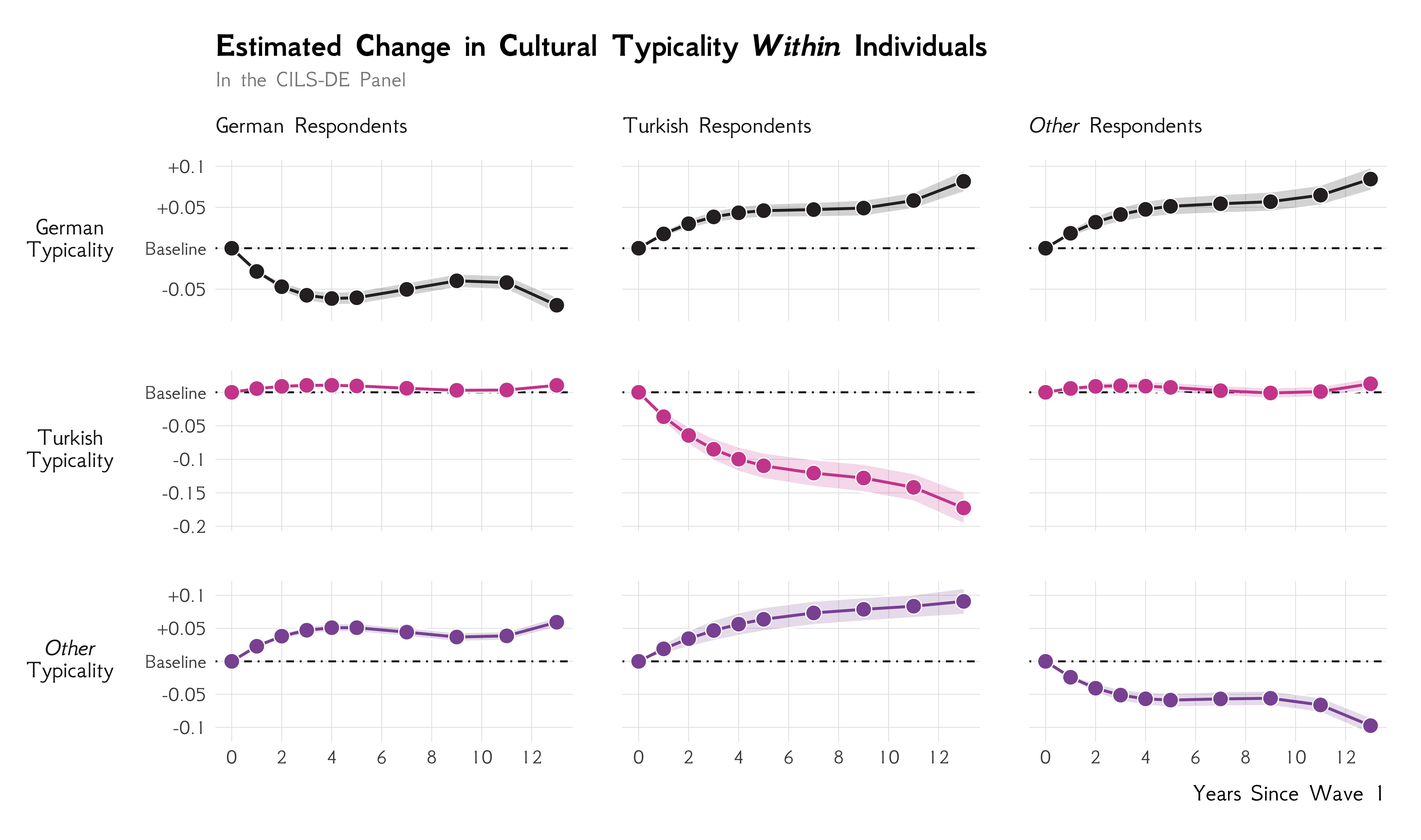
Figure 2  from Karim (2026)

Back to Qualtrics

Refining Your Survey Instrument (Part II)

For the rest of today’s session, please work on your
Qualtrics survey assignment once again.

Enjoy the Weekend

References

Note: Scroll to access the entire bibliography

Boutyline, Andrei, Alina Arseniev-Koehler, and Devin J. Cornell. 2023. “School, Studying, and Smarts: Gender Stereotypes and Education Across 80 Years of American Print Media, 1930–2009†.” Social Forces 102(1):263–86. doi: 10.1093/sf/soac148.

Donoho, David. 2017. “50 Years of Data Science.” Journal of Computational and Graphical Statistics 26(4):745–66. doi: 10.1080/10618600.2017.1384734.

Grimmer, Justin, Margaret E. Roberts, and Brandon M. Stewart. 2021. “Machine Learning for Social Science: An Agnostic Approach.” Annual Review of Political Science 24(1):395–419. doi: 10.1146/annurev-polisci-053119-015921.

Hippel, Paul von. 2015. “Linear vs. Logistic Probability Models: Which Is Better, and When?” Statistical Horizons.

Karim, Sakeef M. 2026. “‘A Spectral Vision of Acculturative Change’.”

Llaudet, Elena, and Kōsuke Imai. 2023. Data Analysis for Social Science: A Friendly and Practical Introduction. Princeton (N.J.) Oxford: Princeton University press.

Lundberg, Ian, Jennie E. Brand, and Nanum Jeon. 2022. “Researcher Reasoning Meets Computational Capacity: Machine Learning for Social Science.” Social Science Research 108:102807. doi: 10.1016/j.ssresearch.2022.102807.

Mittleman, Joel. 2022. “Intersecting the Academic Gender Gap: The Education of Lesbian, Gay, and Bisexual America.” American Sociological Review 87(2):303–35. doi: 10.1177/00031224221075776.

Molina, Mario, and Filiz Garip. 2019. “Machine Learning for Sociology.” Annual Review of Sociology 45(Volume 45, 2019):27–45. doi: 10.1146/annurev-soc-073117-041106.

van Loon, Austin. 2022. “Machine Learning and Deductive Social Science: An Introduction to Predictability Hypotheses.”